Trapezoidal Integral Rule Using C++
Starting from the geometrical interpretation of the definite integral, as the net signed area bounded by the integrand \(f(x)\), the x-axis, and the vertical lines \(x = a\) and \(x = b\), the simplest approach to a practical quadrature algorithm is to replace the graph of the integrand by polygonal line defined by a fine number of integrand values to sum the trapezoidal areas formed thereby.
To sample the integration interval \([a,b]\) uniformly, on can be choose equidistant points,
\begin{equation} x_i = a + (i-1)h, i =1,2,…,n \end{equation}
defined by the spacing
\begin{equation} h = (b - a) / (n-1) \end{equation}
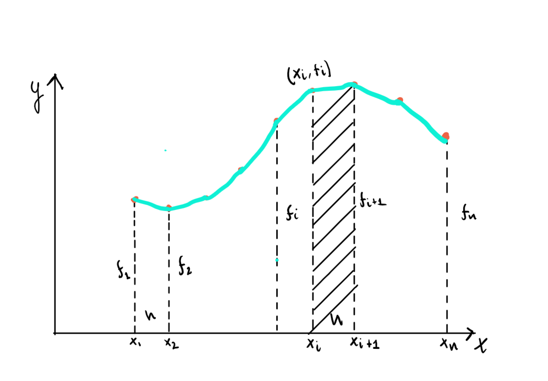 The integrand’s graph is approximated by the line segments connecting the points \((x_i, f_i)\).
Replacing the particle integrals on each of the \((n-1)\) subintervals \((x_i,x_i+1)\) by the corresponding trapezoidal areas, the integral is approximated by
The integrand’s graph is approximated by the line segments connecting the points \((x_i, f_i)\).
Replacing the particle integrals on each of the \((n-1)\) subintervals \((x_i,x_i+1)\) by the corresponding trapezoidal areas, the integral is approximated by
\begin{equation} \int_{a}^{b} f(x) dx \approx \frac{h}{2} (f_1 + f_2) + \cdots+ \frac{h}{2} (f_i + f_{i+1}) + \cdots + \frac{h}{2} (f_{n-1 + f_n}) \end{equation}
and, by further grouping the terms, one obtains the trapezoidal rule:
\begin{equation} \int_{a}^{b} f(x) \approx = h[\frac{f_1}{2} + \sum_{i = 2}^{n - 1} f_i + \frac{f_n}{2}] \end{equation}
#include <iostream>
#include <cmath>

using namespace std;
double  Func(double x)
{
    return (x * x * x) * exp(-x);
}

double Trapezoidal(double  (*Func)(double ), double a, double b, int n)
{
    auto h = (b - a) / (n - 1);

    auto s = 0.5 * (Func(a) + Func(b));
    for (int i = 0; i < n - 1; ++i)
    {
        s += Func(a + i * h);
    }
    return h * s;
}

int main(int argc, char const *argv[])
{
    double a = 0.0, b = 1.0;
    int n = 100;
    cout << "I = " << Trapezoidal(Func, a, b, n) << endl;
    return 0;
}
To evalute the integral test
\begin{equation} \int_{0}^{1} x^3 e^{-x} dx = 0.113935… \end{equation}